Attaching package: 'kableExtra'

The following object is masked from 'package:dplyr':

    group_rows
#Read the penguins_samp1 data file from githubpenguins <-read_csv("https://raw.githubusercontent.com/mcduryea/Intro-to-Bioinformatics/main/data/penguins_samp1.csv")
Rows: 44 Columns: 8
── Column specification ────────────────────────────────────────────────────────
Delimiter: ","
chr (3): species, island, sex
dbl (5): bill_length_mm, bill_depth_mm, flipper_length_mm, body_mass_g, year

ℹ Use `spec()` to retrieve the full column specification for this data.
ℹ Specify the column types or set `show_col_types = FALSE` to quiet this message.
#See the first six rows of the data we've read in to our notebookpenguins %>%head(2) %>%kable() %>%kable_styling(c("striped", "hover"))
species
island
bill_length_mm
bill_depth_mm
flipper_length_mm
body_mass_g
sex
year
Gentoo
Biscoe
59.6
17
230
6050
male
2007
Gentoo
Biscoe
48.6
16
230
5800
male
2008
You can add options to executable code like this
[1] 4
The echo: false option disables the printing of code (only output is displayed).
About Our Data
The data we are working with is a dataset on Penguins, which includes 8 features measured on 44 penguins. The features included are physiological features (like bill length, bill depth, flipper length, body mass, etc) ass well as other features like the year that the penguin was observed,the island the penguins was observed on, the sex of the penguin,and the species of the penguin.
Interesting Questions to Ask
What is the average flipper length? What about for each species?
Are there more male or female penguins? What about per island or species?
What is the average body mass? What about by island? By species? By sex?
What is the ratio of bill length to bill depth for a penguin? What is the overall average of this metric? Does it change by species, sex, or island?
Does average body mass change year?
Data Manipulation Tools and Strategies
We can look at individual columns in a data set or subsets of columns in a dataset. For example, if we are only interested in flipper length and species we can select() those columns
If we want to filter() and only show certain rows, we can do that too.
penguins %>%filter(species =="Chinstrap")
# A tibble: 2 × 8
species island bill_length_mm bill_depth_mm flipper_le…¹ body_…² sex year
<chr> <chr> <dbl> <dbl> <dbl> <dbl> <chr> <dbl>
1 Chinstrap Dream 55.8 19.8 207 4000 male 2009
2 Chinstrap Dream 46.6 17.8 193 3800 fema… 2007
# … with abbreviated variable names ¹flipper_length_mm, ²body_mass_g
#We can also filter by nymerical variablespenguins %>%filter(body_mass_g >=6000)
# A tibble: 2 × 8
species island bill_length_mm bill_depth_mm flipper_leng…¹ body_…² sex year
<chr> <chr> <dbl> <dbl> <dbl> <dbl> <chr> <dbl>
1 Gentoo Biscoe 59.6 17 230 6050 male 2007
2 Gentoo Biscoe 49.2 15.2 221 6300 male 2007
# … with abbreviated variable names ¹flipper_length_mm, ²body_mass_g
#We can also do both penguins %>%filter((body_mass_g >=6000) | (island =="Torgersen"))
# A tibble: 7 × 8
species island bill_length_mm bill_depth_mm flipper_l…¹ body_…² sex year
<chr> <chr> <dbl> <dbl> <dbl> <dbl> <chr> <dbl>
1 Gentoo Biscoe 59.6 17 230 6050 male 2007
2 Gentoo Biscoe 49.2 15.2 221 6300 male 2007
3 Adelie Torgersen 40.6 19 199 4000 male 2009
4 Adelie Torgersen 38.8 17.6 191 3275 fema… 2009
5 Adelie Torgersen 41.1 18.6 189 3325 male 2009
6 Adelie Torgersen 38.6 17 188 2900 fema… 2009
7 Adelie Torgersen 36.2 17.2 187 3150 fema… 2009
# … with abbreviated variable names ¹flipper_length_mm, ²body_mass_g
Answering Our Questions
Most of our questions involve summarizing data, and perhaps summarizing over groups. We can summarize data using the summarize() functions, and data group using group_by().
Let’s find the average flipper length.
#Overall average flipper lengthpenguins %>%summarize(avg_flipper_length =mean(flipper_length_mm))
# A tibble: 3 × 2
  species   av_flipper_length
  <chr>                 <dbl>
1 Adelie                 189.
2 Chinstrap              200
3 Gentoo                 218.
How many of each species do we have?
penguins %>%count(species)
# A tibble: 3 × 2
  species       n
  <chr>     <int>
1 Adelie        9
2 Chinstrap     2
3 Gentoo       33
How many of each sex are there? What about island or species?
penguins %>%count(sex)
# A tibble: 2 × 2
  sex        n
  <chr>  <int>
1 female    20
2 male      24
penguins %>%group_by(species) %>%count(sex)
# A tibble: 6 × 3
# Groups:   species [3]
  species   sex        n
  <chr>     <chr>  <int>
1 Adelie    female     6
2 Adelie    male       3
3 Chinstrap female     1
4 Chinstrap male       1
5 Gentoo    female    13
6 Gentoo    male      20
We can mutate() to add new columns to our data set
# A tibble: 3 × 2
   year mean_body_mass
  <dbl>          <dbl>
1  2007          5079.
2  2008          4929.
3  2009          4518.
Data Visualization:
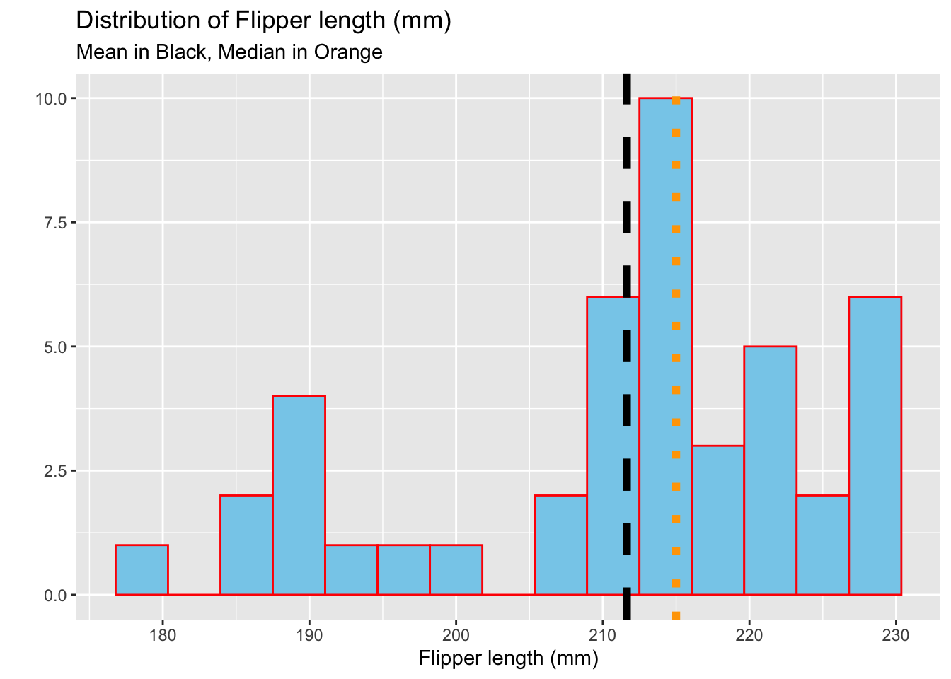
What is the distribution of penguins flipper lengths? numerical
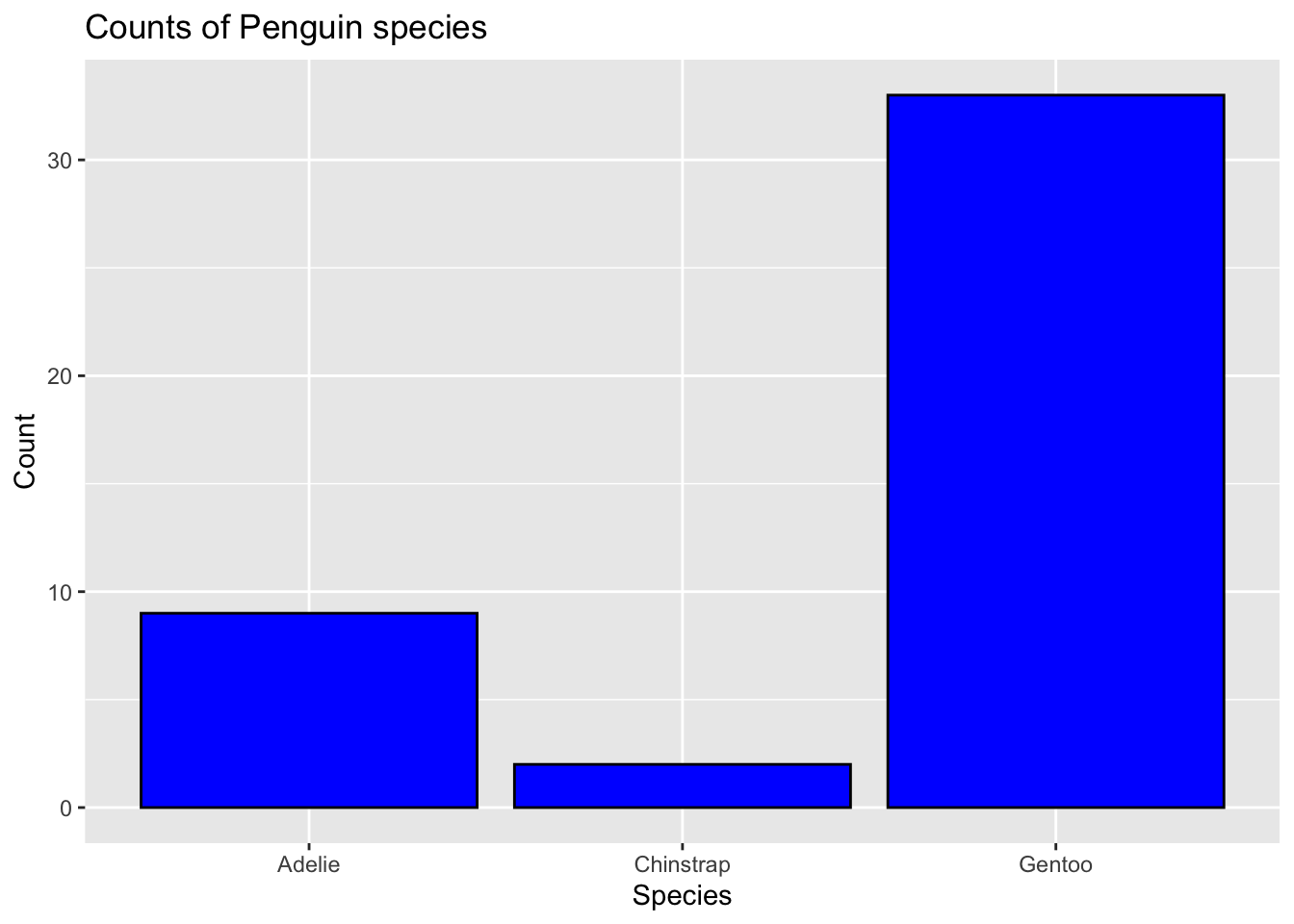
What is the distribution of penguin species? categorical
Does the distribution of flipper length depend of the species of penguins?
How does bill length change throughout the years
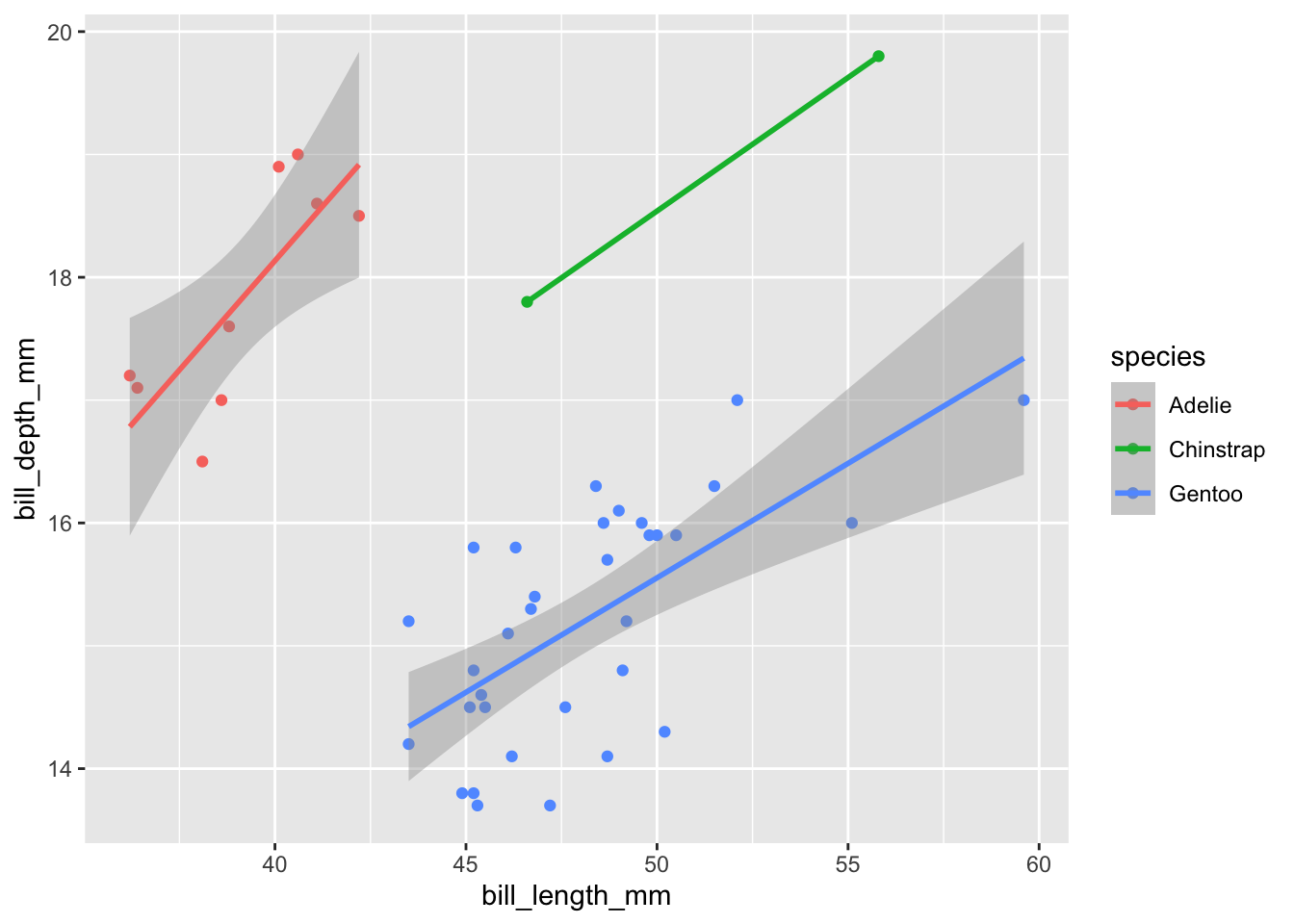
Is there any correlation between the bill length and bill depth? scatterplot
penguins %>%ggplot () +geom_histogram( aes(x = flipper_length_mm), bins =15, fill ="skyblue",color ="red") +labs(title ="Distribution of Flipper length (mm)",subtitle ="Mean in Black, Median in Orange",y ="", x ="Flipper length (mm)") +geom_vline(aes (xintercept =mean (flipper_length_mm)), lwd =2, lty ="dashed" ) +geom_vline(aes (xintercept =median (flipper_length_mm)),color ="orange", lwd =2, lty ="dotted")
Warning: Using `size` aesthetic for lines was deprecated in ggplot2 3.4.0.
ℹ Please use `linewidth` instead.
Categorical Plot
penguins %>%ggplot() +geom_bar(mapping =aes(x = species ), color ="black", fill="blue") +labs(title ="Counts of Penguin species",x ="Species", y ="Count")
Let’s make a scatter plot see if bill legnth is correlated with bill depth
penguins %>%ggplot() +geom_point(aes(x = bill_length_mm, y = bill_depth_mm, color = species)) +geom_smooth(aes(x =bill_length_mm, y = bill_depth_mm, color = species), method ="lm")
`geom_smooth()` using formula = 'y ~ x'
Warning in qt((1 - level)/2, df): NaNs produced
Warning in max(ids, na.rm = TRUE): no non-missing arguments to max; returning
-Inf
Whether the average length for a penguin exceeds 45mm?
t.test (penguins$bill_length_mm, alternative ="greater", mu =45, corf.level =0.95)
    One Sample t-test

data:  penguins$bill_length_mm
t = 1.8438, df = 43, p-value = 0.03606
alternative hypothesis: true mean is greater than 45
95 percent confidence interval:
 45.12094      Inf
sample estimates:
mean of x
 46.37045
Notes:
Revisiting Intro Stats
We assumed the Central Limit Theorem. The sampling distribution tends toward a normal distribution as sample sizes get larger.
Simulation-based Methods
Assumption: our data is randomly sampled and is representative of our population.
Bootstrapping; Treating our sample as if it were the population.